Tutorial 1: a first ACE fit for silicon

In this notebook you build an ACE basis, fit a linear ACE model to a small silicon dataset, check it on test data, and then use it as an ASE calculator for an equation of state and a short molecular-dynamics run. Everything runs on a CPU in a few minutes.

Goals

1. Build an ACE basis and know what order and max_degree control.
2. Fit it with ace-jax's evidence-based linear fit, and read the test metrics.
3. Judge the fit with a parity plot, not just an RMSE.
4. Use the fitted model in ASE: an equation of state and NVE molecular dynamics.

Each step ends with a checkpoint cell that tells you whether the step worked. The exercises at the end change one thing at a time; the notebook re-runs only what depends on the change.

Run this notebook. Install uv. Then run this command:

uvx marimo edit --sandbox https://raw.githubusercontent.com/ACEsuit/ace-jax/main/docs/user/tutorials/notebooks/first_fit_si.py

The notebook opens in your browser. You do not need an account. You can also open the notebook in molab, the marimo hosted service. You must sign in to run it there.

This website shows a static copy of the notebook, run on a CPU when the site was built. The interactive controls show their default values. Run time: approximately 1 minute (the fit takes approximately 30 s).

import os
import pathlib
import time
import urllib.request

import jax

jax.config.update("jax_enable_x64", True)  # fitting needs float64

import marimo as mo
import matplotlib.pyplot as plt
import numpy as np
from ase.io import read, write

import ace_jax as aj
from ace_jax import ACECalculator

Step 1: the data

si_tiny_train.xyz is a 53-configuration silicon dataset from the ace-jax test fixtures: 2-atom diamond and β-tin cells, two 64-atom liquid snapshots and one isolated atom, labelled with DFT. The labels are stored under dft_energy, dft_force and dft_virial.

The cell below uses the copy in your ace-jax checkout if this notebook is run from one, and otherwise downloads it from GitHub.

work = pathlib.Path("ace_jax_tutorial_1")
work.mkdir(exist_ok=True)
URL = "https://raw.githubusercontent.com/ACEsuit/ace-jax/main/fixtures/si_tiny_train.xyz"
_local = mo.notebook_dir() / "../../../../fixtures/si_tiny_train.xyz" if mo.notebook_dir() else None
data_file = work / "si_tiny_train.xyz"
if _local is not None and _local.exists():
    data_file.write_bytes(_local.read_bytes())
elif not data_file.exists():
    urllib.request.urlretrieve(URL, data_file)
keys = dict(energy_key="dft_energy", force_key="dft_force", virial_key="dft_virial")

frames = read(data_file, ":")
_kinds = {}
for _a in frames:
    _kinds.setdefault(_a.info["config_type"], []).append(len(_a))
# Leave the isolated atom out: its energy is the reference energy E0 itself,
# and the fit below determines E0 from the bulk energies (e0="lsq").
bulk_frames = [_a for _a in frames if _a.info["config_type"] != "isolated_atom"]
train_file, test_file = work / "train.xyz", work / "test.xyz"
write(test_file, bulk_frames[::4])
write(train_file, [_a for _i, _a in enumerate(bulk_frames) if _i % 4])
mo.md(
    "| config_type | configs | atoms each |\n|---|---|---|\n"
    + "\n".join(f"| `{k}` | {len(v)} | {sorted(set(v))} |" for k, v in _kinds.items())
    + f"\n\nTraining set: **{len(bulk_frames) - len(bulk_frames[::4])}** configs, "
    f"test set: **{len(bulk_frames[::4])}** configs (every fourth bulk config)."
)

config_type	configs	atoms each
isolated_atom	1	[1]
dia	25	[2]
bt	25	[2]
liq	2	[64]

Training set: 39 configs, test set: 13 configs (every fourth bulk config).

Step 2: build a basis

An ACE basis is set by the elements, the correlation order (how many neighbours each basis function couples; order 3 means four-body terms) and the maximum total degree, which bounds the polynomial degree and so the basis size. radial_mode="onehot" (the default) uses the radial polynomials themselves as the radial basis.

BasisSpec describes the basis and build_basis builds it; the first build of a new shape computes its coupling coefficients (milliseconds) and caches them. On the command line, aj fit --order 3 --max-degree 10 ... builds the same basis inside the fit, and aj basis saves one on its own.

max_degree = mo.ui.dropdown(options=["8", "10", "12"], value="10", label="max degree")
radial_mode = mo.ui.dropdown(options=["onehot", "glorot_normal"], value="onehot", label="radial mode")
mo.hstack([max_degree, radial_mode], justify="start")

Interactive controls in the notebook (this page shows their defaults): max degree = 10, radial mode = onehot

from ace_jax.basis.model import BasisSpec, build_basis

spec = BasisSpec(order=3, max_degree=int(max_degree.value), elements=("Si",),
                 radial_mode=radial_mode.value)
basis = build_basis(spec)
mo.md(f"Basis: **{basis.meta['len_basis']}** functions ({basis.meta['n_B']} many-body, "
      f"{basis.meta['n_pair']} pair), cutoff {basis.meta['rcut']} Å")

Basis: 120 functions (110 many-body, 10 pair), cutoff 5.5 Å

Step 3: fit

aj fit and the Python pipeline below solve the same problem: Bayesian linear regression of the energies, forces and virials on the basis. The noise levels of the three quantities and the prior scale of the coefficients are not hand-tuned weights: they are chosen by maximising the evidence (the marginal likelihood), here with L-BFGS.

The command-line equivalent is

aj fit --order 3 --max-degree 10 --train train.xyz --test test.xyz \
    --energy-key dft_energy --force-key dft_force --virial-key dft_virial \
    --e0 lsq --m-per-species 0 --opt lbfgs --out fit

FitConfig(model=...) takes the Basis built above, a BasisSpec (built inside the fit from the species in the data) or the path of a saved basis file. r0=None centres the hyperprior on the basis's mean bond length, as the command line does.

from ace_jax.fit.pipeline import FitConfig, fit, load_fit_data, save_model

_t = time.time()
cfg = FitConfig(model=basis, arm="linear", m_per_species=0, e0="lsq",
                opt="lbfgs", r0=None, rungs=("map",), predict_stats="recompute", predict_train=False,
                **keys).validate()
_data = load_fit_data(cfg, train=str(train_file), test=str(test_file))
result = fit(cfg, _data)
model_file = save_model(result, work / "fit")
fit_seconds = time.time() - _t
test_metrics = result.preds.metrics["test/map"]
mo.md(
    f"Fitted in {fit_seconds:.0f} s → `{model_file}`\n\n"
    "| quantity | test RMSE | coverage (±1σ) |\n|---|---|---|\n"
    + "\n".join(f"| {q} ({u}) | {test_metrics[q]['rmse']:.4g} | {test_metrics[q]['coverage']:.2f} |"
                for q, u in (("E", "meV/atom"), ("F", "eV/Å"), ("V", "eV")))
)

  lbfgs start 0 eval 1  logpost = -28476.8  (0 s)
  lbfgs start 0 eval 2  logpost = -3364.11  (0 s)
  lbfgs start 0 eval 3  logpost = -3262.51  (0 s)
  lbfgs start 0 eval 4  logpost = -2857.51  (0 s)
  lbfgs start 0 eval 5  logpost = -1296.41  (0 s)
  lbfgs start 0 eval 6  logpost = -1.47134e+09  (0 s)
  lbfgs start 0 eval 7  logpost = -8043.61  (0 s)
  lbfgs start 0 eval 8  logpost = -740.346  (0 s)
  lbfgs start 0 eval 9  logpost = -2794.11  (0 s)
  lbfgs start 0 eval 10  logpost = -496.002  (0 s)
  lbfgs start 0 eval 11  logpost = -670.009  (0 s)
  lbfgs start 0 eval 12  logpost = -421.171  (0 s)
  lbfgs start 0 eval 13  logpost = -372.082  (0 s)
  lbfgs start 0 eval 14  logpost = -290.715  (0 s)
  lbfgs start 0 eval 15  logpost = -264.442  (0 s)
  lbfgs start 0 eval 16  logpost = -257.089  (0 s)
  lbfgs start 0 eval 17  logpost = -255.741  (0 s)
  lbfgs start 0 eval 18  logpost = -255.632  (0 s)
  lbfgs start 0 eval 19  logpost = -255.557  (0 s)
  lbfgs start 0 eval 20  logpost = -255.472  (0 s)
  lbfgs start 0 eval 21  logpost = -255.471  (0 s)
  lbfgs start 0 eval 22  logpost = -255.471  (0 s)
  lbfgs start 0 eval 23  logpost = -255.471  (0 s)
L-BFGS start 0: logpost -255.471  nfev 23  CONVERGENCE: RELATIVE REDUCTION OF F <= FACTR*EPSMCH
L-BFGS: best of 1 start(s) = start 0, logpost -255.471
Newton polish (exact Hessian, column-wise HVPs): converged (|pg| 1.30e-11 within 10x the gradient roundoff 4.3e-11); 5 step(s), 6 Hessian(s), 60 HVPs, 63 gradient evaluations, 1.8 s
MAP: stationary (predicted gain 3.4e-24 nats), logpost -255.4705441
test map {'E': {'rmse': 22.4313, 'crps': 13.895, 'coverage': 0.1538, 'rho': 0.5769, 'rms_z': 3.7809}, 'F': {'rmse': 0.0975, 'crps': 0.0657, 'coverage': 0.1795, 'rho': 0.3422, 'rms_z': 4.3845}, 'V': {'rmse': 0.2896, 'crps': 0.1681, 'coverage': 0.2308, 'rho': 0.4791, 'rms_z': 3.4612}}
RMSE, test (map)
-----------------------------------------------------------------
config type  configs  atoms  E (meV/atom)  F (eV/Å)  V (meV/atom)
-----------------------------------------------------------------
bt                 6     12         32.23    0.0993        198.91
dia                7     14          6.62    0.0959         70.87
-----------------------------------------------------------------
all               13     26         22.43    0.0975        144.80

Fitted in 20 s → ace_jax_tutorial_1/fit/model.npz

quantity	test RMSE	coverage (±1σ)
E (meV/atom)	22.43	0.15
F (eV/Å)	0.09749	0.18
V (eV)	0.2896	0.23

Checkpoint 1 passed: test force RMSE below 0.2 eV/Å and energy RMSE below 50 meV/atom.

Step 4: parity plot

An RMSE hides where the errors are. Evaluate the fitted model on the test set with the ASE calculator and plot predictions against the labels. skin=0 builds a fresh neighbour list for each structure, the right choice for a set of unrelated structures.

from ase import Atoms

from ace_jax.fit.data import load_configs  # libAtoms extxyz reader: labels as written

calc = ACECalculator(str(model_file), skin=0)
_E_ref, _E_fit, _F_ref, _F_fit = [], [], [], []
for _c in load_configs(str(test_file), **keys):
    _at = Atoms(numbers=_c.numbers, positions=_c.positions, cell=_c.cell, pbc=_c.pbc)
    _at.calc = calc
    _E_ref.append(_c.energy / len(_at)); _E_fit.append(_at.get_potential_energy() / len(_at))
    _F_ref.append(_c.forces.ravel()); _F_fit.append(_at.get_forces().ravel())
parity = {"E_ref": np.array(_E_ref), "E_fit": np.array(_E_fit),
          "F_ref": np.concatenate(_F_ref), "F_fit": np.concatenate(_F_fit)}

_fig, (_a1, _a2) = plt.subplots(1, 2, figsize=(9, 4))
for _ax, _r, _f, _lab in ((_a1, parity["E_ref"], parity["E_fit"], "energy (eV/atom)"),
                          (_a2, parity["F_ref"], parity["F_fit"], "force component (eV/Å)")):
    _lo, _hi = min(_r.min(), _f.min()), max(_r.max(), _f.max())
    _ax.plot([_lo, _hi], [_lo, _hi], "k-", lw=0.8)
    _ax.plot(_r, _f, "o", ms=4, alpha=0.7)
    _ax.set_xlabel("DFT " + _lab); _ax.set_ylabel("ACE " + _lab)
_rmse = 1e3 * np.sqrt(np.mean((parity["E_fit"] - parity["E_ref"]) ** 2))
_a1.set_title(f"E RMSE {_rmse:.1f} meV/atom")
_a2.set_title(f"F RMSE {np.sqrt(np.mean((parity['F_fit'] - parity['F_ref']) ** 2)):.3f} eV/Å")
_fig.tight_layout()
_fig

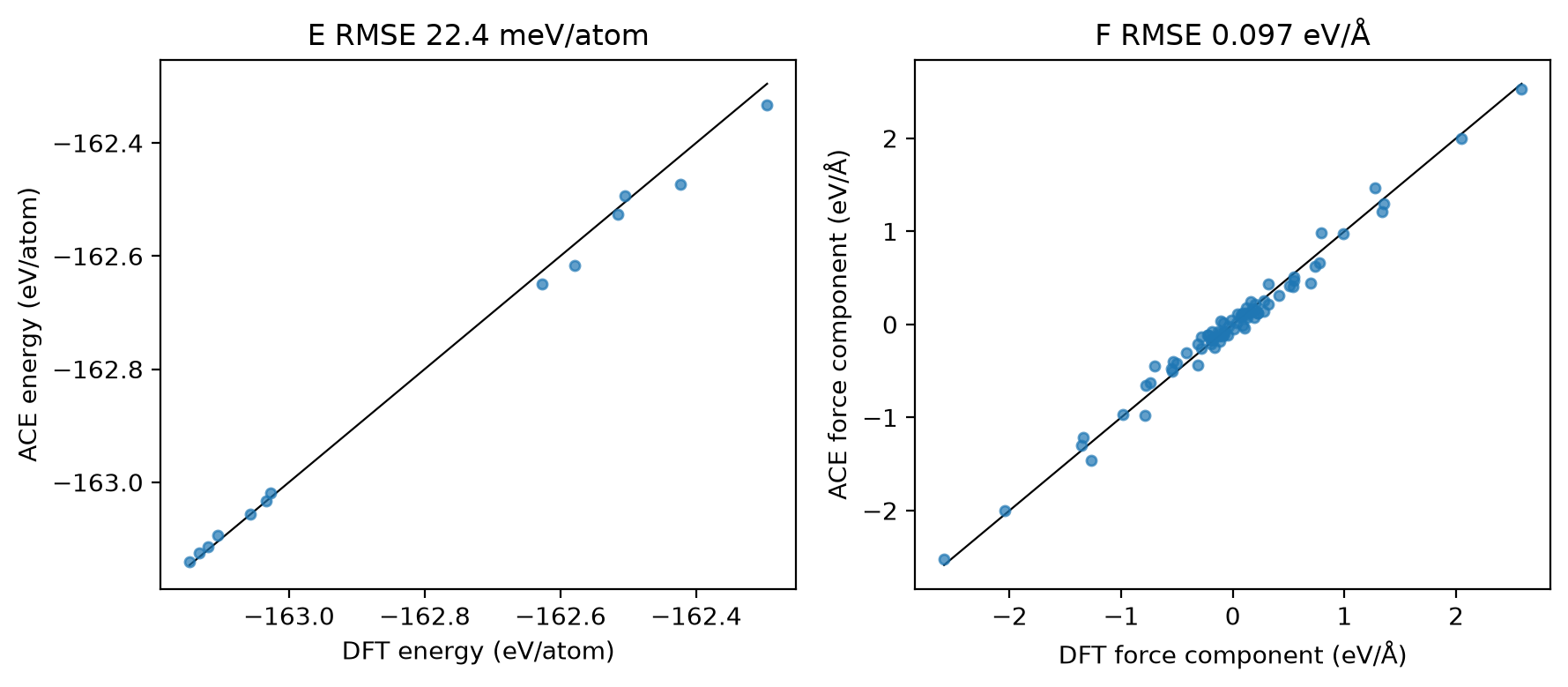
Checkpoint 2 passed: the calculator's energy RMSE (22.431 meV/atom) matches the fit's.

Step 5: equation of state

The training set holds strained diamond and β-tin cells. Scan the volume of the diamond cell and fit a Birch–Murnaghan equation of state. The experimental lattice constant of silicon is 5.43 Å and its bulk modulus about 98 GPa; DFT with this functional gives a slightly larger lattice constant.

from ase.build import bulk
from ase.eos import EquationOfState
from ase.units import GPa

_vols, _ens = [], []
for _a in np.linspace(5.25, 5.65, 9):
    _at = bulk("Si", "diamond", a=_a)
    _at.calc = calc
    _vols.append(_at.get_volume()); _ens.append(_at.get_potential_energy())
_eos = EquationOfState(_vols, _ens, eos="birchmurnaghan")
v0, e0, B = _eos.fit()
a0 = (4 * v0) ** (1 / 3)  # the 2-atom primitive cell holds a quarter of the cubic cell
_fig, _ax = plt.subplots(figsize=(5, 3.5))
_ax.plot(_vols, _ens, "o")
_v = np.linspace(min(_vols), max(_vols), 100)
_ax.plot(_v, _eos.func(_v, *_eos.eos_parameters), "-")
_ax.set_xlabel("volume (ų per 2 atoms)"); _ax.set_ylabel("energy (eV)")
_ax.set_title(f"a0 = {a0:.3f} Å, B = {B / GPa:.0f} GPa")
_fig.tight_layout()
_fig

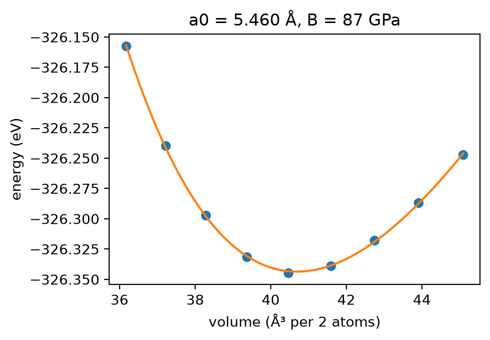
Checkpoint 3 passed: a0 = 5.460 Å and B = 87 GPa are physical for silicon.

Step 6: molecular dynamics

Run 200 steps (0.2 ps) of constant-energy (NVE) dynamics on a 64-atom diamond cell started at 600 K. The calculator keeps a Verlet neighbour list (skin=1.0 Å by default) and rebuilds it only when atoms have moved far enough, so each step is one compiled call. A good potential conserves the total energy.

from ase import units
from ase.md.verlet import VelocityVerlet

try:  # ASE >= 3.29
    from ase.md.velocitydistribution import thermalize_momenta as _thermalize
except ImportError:
    from ase.md.velocitydistribution import MaxwellBoltzmannDistribution as _thermalize

_at = bulk("Si", "diamond", a=5.43, cubic=True).repeat(2)
_at.calc = ACECalculator(str(model_file))
_thermalize(_at, temperature_K=600, rng=np.random.default_rng(0))
_dyn = VelocityVerlet(_at, 1.0 * units.fs)
_etot, _temp = [], []
_dyn.attach(lambda: (_etot.append(_at.get_total_energy()), _temp.append(_at.get_temperature())), interval=5)
_t = time.time()
_dyn.run(200)
md_seconds = time.time() - _t
drift = (max(_etot) - min(_etot)) / len(_at)
_fig, (_a1, _a2) = plt.subplots(1, 2, figsize=(9, 3.5))
_steps = np.arange(len(_etot)) * 5
_a1.plot(_steps, _temp); _a1.set_xlabel("step"); _a1.set_ylabel("T (K)")
_a2.plot(_steps, (np.array(_etot) - _etot[0]) * 1e3 / len(_at))
_a2.set_xlabel("step"); _a2.set_ylabel("E_tot - E_tot(0) (meV/atom)")
_a1.set_title(f"200 steps in {md_seconds:.1f} s, "
              f"{_at.calc.last_timing['rebuilds']} neighbour-list builds")
_fig.tight_layout()
_fig

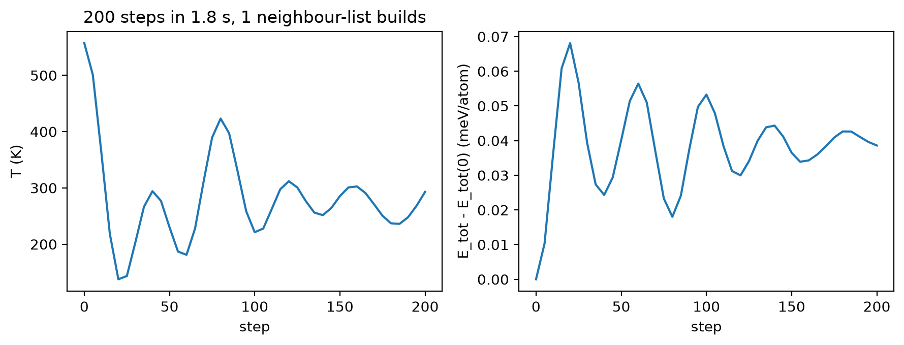
Checkpoint 4 passed: the total energy stays within 0.068 meV/atom over 0.2 ps.

Exercises

1. Basis size. Change max degree to 8 and to 12 in Step 2. How do the basis size and the test errors change? With 39 small training cells, does a bigger basis keep helping? Why is degree 8 so much worse in energy than in forces?
2. Radial basis. Switch radial mode to glorot_normal, which mixes the radial polynomials with seeded random weights. Compare the test errors. Tutorial 2 shows how to learn the radial weights instead of keeping them frozen.
3. E0 and the isolated atom. In Step 1, add the isolated atom (the first frame) to the training set: append + frames[:1] to the list written to train_file. How do the fitted E0 (np.load(...)["E0"] of the saved model) and the test errors change? (Hint: an isolated atom has no neighbours, so its predicted energy is E0 alone.)
4. β-tin. Repeat the equation of state for β-tin (bulk("Si", "beta-tin", a=4.9, c=2.7) is a reasonable start) and compare the two energy minima per atom.

Hint for exercise 1

Degree 8 gives 62 functions, too few to fit energies and forces together: it cannot separate diamond from beta-tin. The evidence then treats the energies as noise (a large result.theta.log_sigma_E, about -1.5 against -4.1 at degree 10) and fits the forces. Test E RMSE: about 180, 22 and 14 meV/atom at degrees 8, 10 and 12.

Hint for exercise 3

An atom with no neighbours is predicted as E0 alone, so with e0='lsq' an isolated atom in the training set sets the E0 of its species to its energy exactly (-158.545 eV here). Without one, E0 is fitted with the model, to -161.90 eV: it is then only a reference level, not a free-atom energy. The bulk is fitted relative to it either way, and the test errors barely move (22 to 24 meV/atom and 0.10 eV/A).

Summary

• build_basis(BasisSpec(...)) (or aj fit --order ... --max-degree ...) makes an unfitted basis; order and max_degree set its size.
• The linear fit picks its own energy/force/virial weights by evidence maximisation; e0="lsq" fits the reference energies.
• ACECalculator turns the fitted model.npz into an ASE calculator that is fast enough for molecular dynamics.

Next: Tutorial 2 learns the radial basis.